Recently I wrote some code to interpolate between 2D polygons. It and all the snippets here are in OpenSCAD, but it’s straightforward to apply elsewhere.
Box to cross to circle to box and around and around we go.
If you want to skip the development details, the code with simple API wrappers is included in my open source OpenSCAD utilities library.
Utilities
At various points below the following debug, convenience, and sub-functions are used.
A debug utility to outline a polygon with red dots at its vertices:
module outline(a, n=1, col="red", d=1, fill=true) {
  if (fill)
    polygon(a);

  for (p = [0 : n : len(a)-1])
    translate([a[p].x, a[p].y, 0])
      color(col)
      sphere(d=d);
}
A convenience function to calculate the distance between two points:
function dist(a, b) = sqrt((b.x-a.x)^2 + (b.y-a.y)^2);
A sub-function to recursively compute the length of the perimeter of a polygon:
function perimeter(a, i=0) =
  (i == len(a)-1)
  ? dist(a[i], a[0])
  : dist(a[i], a[i+1]) + perimeter(a, i+1);
Interpolation
Interpolating between two polygons with an equal number of points is a simple application of linear algebra. Given two matrices A and B representing the points and a scalar k capturing the desired bias from A (k=0) to B (k=1), the interpolation is simply (1-k)A+kB. Think of it as adding together each x and y component of each point from both polygons, applying k as a sliding value from A on the left (0) to B on the right (1) denoting how much to take from one or the other. This is very simple in OpenSCAD:
function interp(a, b, bias) = (1-bias)*a + bias*b;
The cute part in practice then is deriving polygons with an equal number of points.
Generation and Alignment
Before doing that, the vertices of the polygons also need to be mapped. There could be an explicit mapping, or one based on distance, or some other mechanism. Here it is simply assumed that the vertex lists are matched, i.e., each successive pair of points drawn one from each polygon is to be mapped to each other. An easy way to do this is to generate the lists of vertices such that they start at the same absolute angle, e.g., 0°, and proceed in the same rotational direction. Without such matching the interpolations below will rotate the derived shape as it morphs between the start and end, which can be cool but is not desired in all cases.
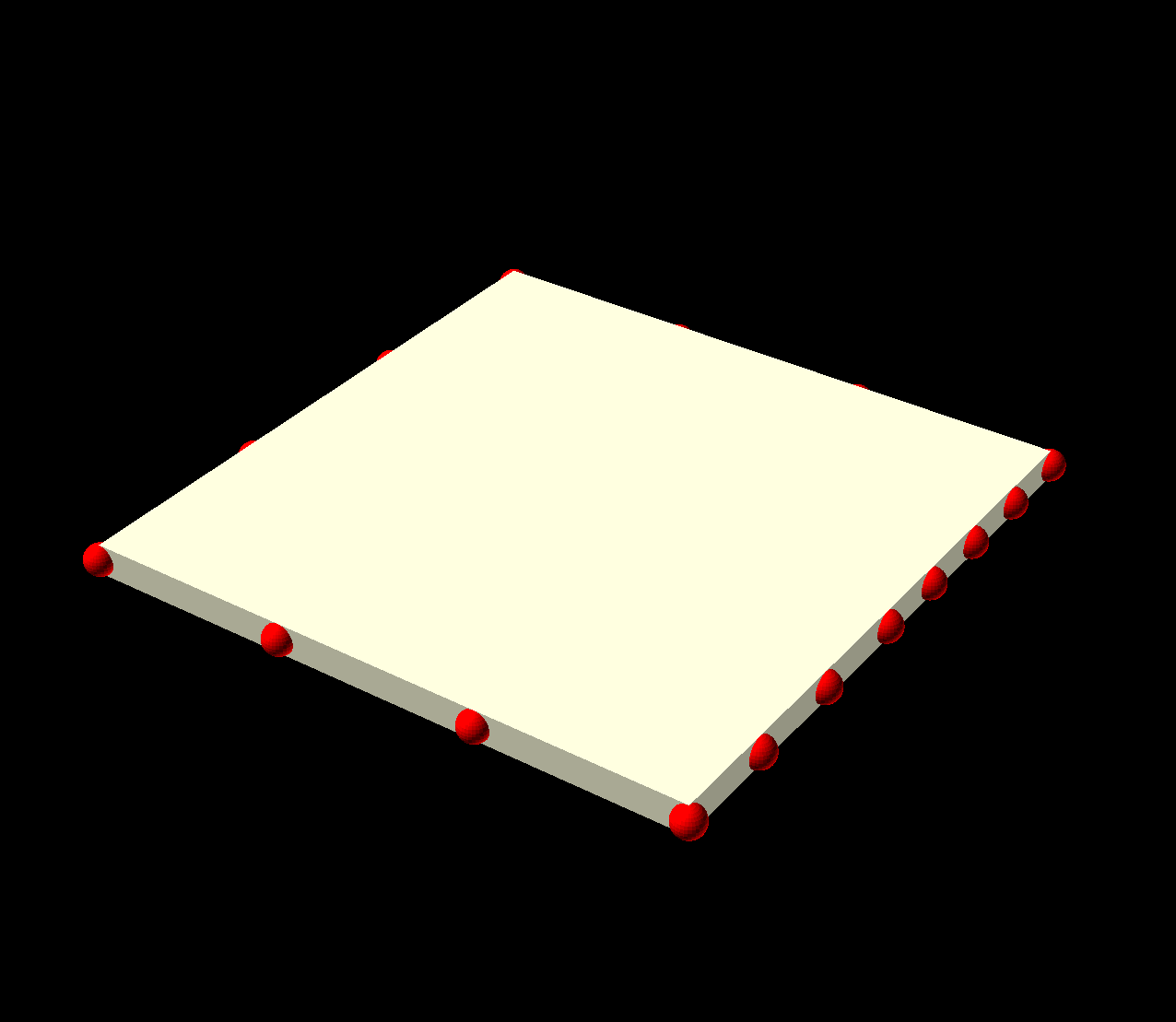
For an example polygon, the box used here is generated as five points:
function box(r) =
  [
    [r, 0],
    [r, r],
    [-r, r],
    [-r, -r],
    [r, -r]
  ];
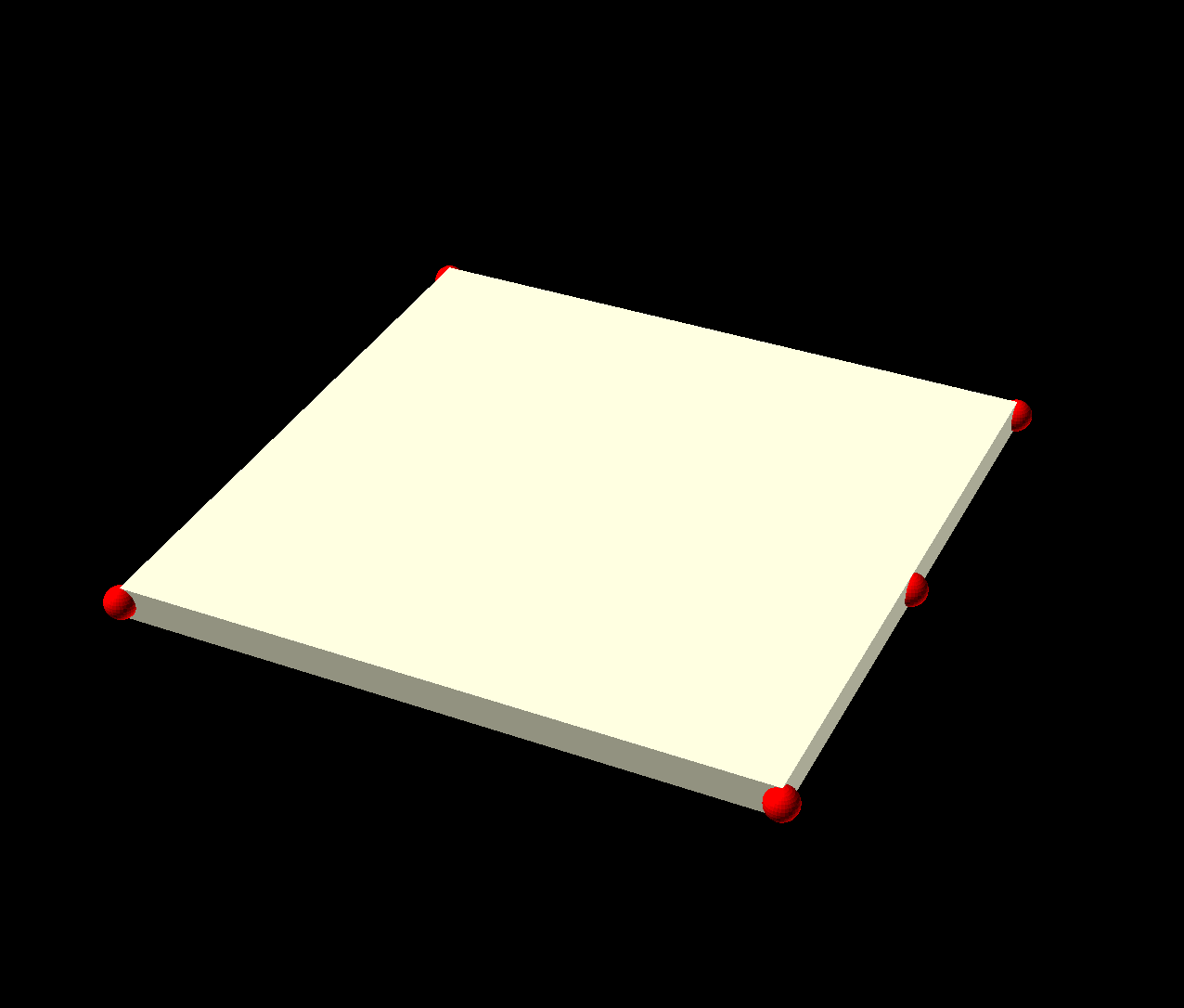
Box generated as five points.
The extra fifth point is so that there’s an initial 0th point at 0° from the center, [r, 0]. It doesn’t need to be on that angle but starting from 0° is a simple convention that makes it easier to align a variety of shape generators. If each started at a point more natural to its shape, e.g., the upper right corner of the box, either the interpolations would rotate, or a lot more work would be required to align them.
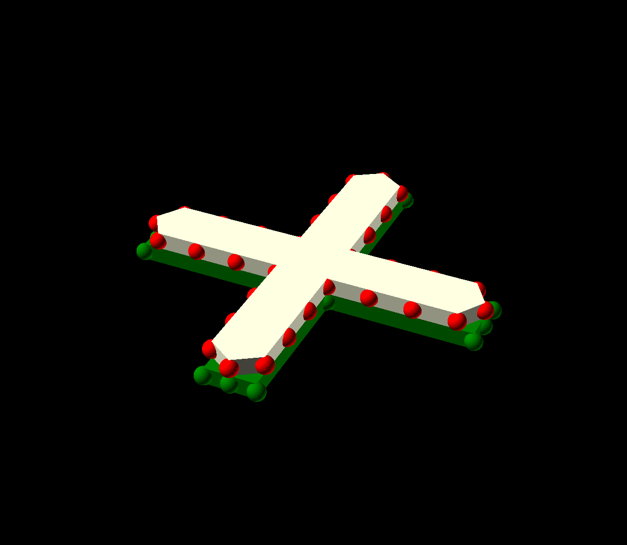
The cross in these examples is generated as sixteen points:
function cross(r, w) =
  let (y = min(r/2, w/2),
       a = asin(y/r),
       x = cos(a) * r
       )
  [
    [x, 0],
    [x, y],
    [y, y],
    [y, x],
    [0, x],
    [-y, x],
    [-y, y],
    [-x, y],
    [-x, 0],
    [-x, -y],
    [-y, -y],
    [-y, -x],
    [0, -x],
    [y, -x],
    [y, -y],
    [x, -y],
  ];
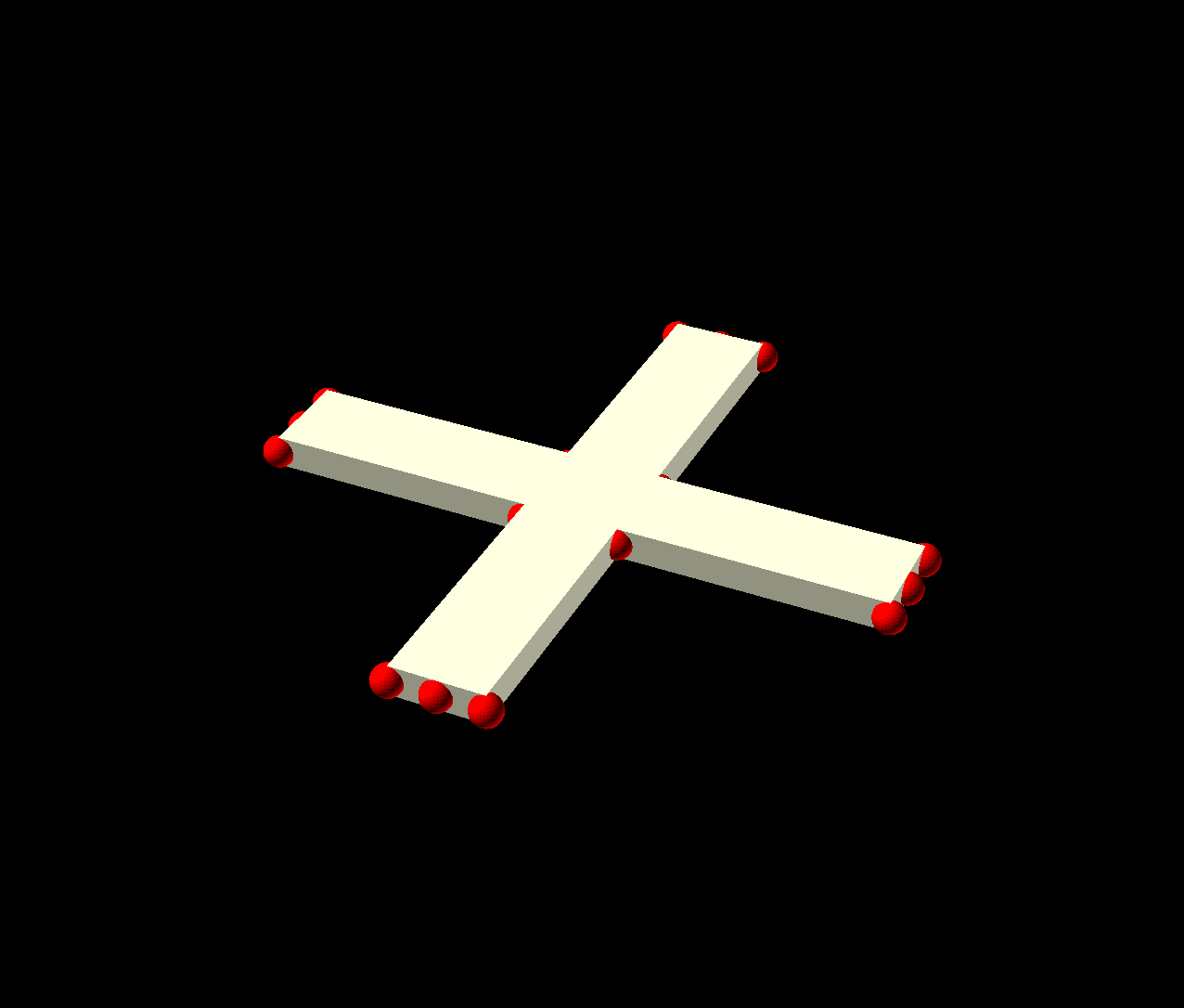
Cross generated as 16 points.
Similarly to the box, there’s an extra point at the middle of the cross arm’s outer edge so that the shape starts at 0°, [r, 0]. This particular generator produces this middle point for each arm, but there’s no particular need for that. The trigonometry at the top of the function is for later use, to treat the parameter r as the radius of a circle in which the cross is to be inscribed rather than the length of the arms directly.
Circles are approximated by a given number of rays, again starting from 0°:
function circlepts(n, r) = [
                            for (a=[0:n-1])
                              [
                               cos(a*360/n) * r, sin(a*360/n) * r
                              ]
                           ];
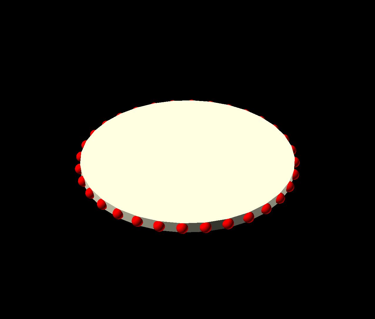
Circle generated as 32 points.
Approach 1: Duplication
With two polygons aligned by mapped initial points, in this case at 0° for convenience, we next need to extend them to the same number of points. A degenerate but workable way to do this is to duplicate the vertices of the lesser polygon as necessary. The slight subtlety is that the number of points must be exactly max(|A|, |B|). This function manages that by explicitly accounting for the fractional difference between the matrix dimensions of the polygons, allocating the extra points uniformly by count:
function poly_dupe(q, n) =
  let (
       midpts = floor(n/len(q)),
       excess = n % len(q)
       )
  [ for (seg = [0:len(q)-1])
      let (
           p = q[seg],
           k = midpts + ((seg < excess)? 1 : 0)
           )
	for (i = [0:k-1])
          p
    ];
This works technically, but unsurprisingly the results are not satisfactory.

Interpolating between polygons via simple duplication.
Approach 2: Uniform Subdivision
The problem in the previous simple duplication is that the shapes are being morphed solely at the vertices rather than all along the edges. The interpolation is too coarse. This can be mitigated by extending the lesser polygon with additional derived points along its edges. This function does so while allocating the additional points to each edge as uniformly as possible by count (as opposed to by geometric distance):
function poly_resample_uniform(q, n) =
  (perimeter(q) <= 0)
  ? poly_dupe(q, n)
  : let (
         midpts = floor(n/len(q)),
         excess = n % len(q)
         )
  [ for (seg = [0:len(q)-1])
      let (
           p1 = q[seg],
           k = midpts + ((seg < excess)? 1 : 0)
           )
        for (i = [0:k-1])
          let (
               p2 = q[(seg+1)%len(q)],

               dx = p2.x - p1.x,
               dy = p2.y - p1.y,
               d = sqrt(dx^2 + dy^2)
               )
            [p1.x+dx*i/k, p1.y+dy*i/k]
    ];
This works better but still not great:
One way of looking at the problems is that adding points uniformly by the number of edges doesn’t account for the edges being of varying length. Shorter edges are thus sampled at higher frequency compared to the others, so their interpolation is a better approximation. In this case, the right side has additional points that don’t need to move nearly as much as those on the more grossly approximated other sides to reach their final position, so the shape doesn’t morph evenly visually.
Uniform allocation by count of additional points.
Approach 3: Resampling
That need for higher sampling and better approximation of the longer edges could be addressed by resampling the lesser polygon to distribute points evenly by distance around its perimeter. This could be done a couple ways; this function uses a two-step recursion to iterate over edges and points to be generated, advancing the sampling point along the original shape a uniform fraction of the total perimeter:
function poly_resample(q, n) =
  let (
       per = perimeter(q)
       )
  (per <= 0)
  ? poly_dupe(q, n)
  : poly_resample_(q, 0, 0, n, 0, per);

function poly_resample_(q, e, i, n, per_acc, per) =
  let (
       p1 = q[e],
       p2 = q[(e+1)%len(q)],

       dx = p2.x - p1.x,
       dy = p2.y - p1.y,
       d = sqrt(dx^2 + dy^2),

       per_i = i/n * per,
       frac = (per_i-per_acc)/d,

       p = [p1.x+dx*frac, p1.y+dy*frac]
       )
  (per_i >= per_acc+d)
  ? poly_resample_(q, e+1, i, n, per_acc+d, per)
  : (i < n-1)
  ? concat([p], poly_resample_(q, e, i+1, n, per_acc, per))
  : [p];
This works great for some shapes and point counts, e.g., the box and cross.

Interpolating the shapes by resampling the box.
However, the approximation produces artifacts in some combinations of shapes and points. For example, in interpolating between the circle and cross, resampling the cross to match the circle’s point count causes the ends of its arms to lose their sharp corners.

Morphing between a circle and a cross.
It turns out that when the cross is resampled to have 32 points (and other sizes), the corners are deformed because the resampling averages them inward. With more points the approximation is better and the effect less noticeable, but this is not ideal.
Cross resampled to have 32 points.
Approach 4: Proportional Subdivision
What’s necessary is to retain the original vertices, preserving the true outline, but subdivide the edges with additional points proportional to the edges’ lengths relative to the total perimeter. This seems tricky because of the need to derive exactly max(|A|, |B|) points. It’s not clear to me that there is a simple local calculation per edge that can do so while appropriately accounting for the fractional difference between the point counts, which seems to require comparison across all the edge lengths.
In any event, here this is performed by allocating each edge a number of points based on its length’s percentage of the polygon’s perimeter and the total number of points to derive, with a minimum of one. Necessarily flooring those allocations to an integer, for a discrete number of points, can result in undercounting. Conversely, the minimum of one, which is required in order to capture each edge, can result in overcounting. So the initial allocations are then adjusted to add or take away the necessary number of allocations, one each per edge in order of descending length. The intuition is that if points are being added, longer edges can use a finer approximation, while if points are being removed, longer edges can stand a coarser approximation.
That adjustment is performed by creating a list of tuples capturing the index and length of each edge. This is sorted in descending order by edge length and that list in turn iterated over the necessary number of adjustments, using the indexes to bump the allocations up or down as appropriate for the longest edges. Working within OpenSCAD’s mostly functional paradigm, the latter is done via constructing another helper structure comprised of a list of tuples with edges indexes and their allocations. That second structure is then sorted by the edge indexes and read out to get the final allocations in edge sequence order. From there the subdivision is a simple matter of iterating over the edges and evenly sampling the allocated number of points for each.
The code begins with the two sorting functions:
function qsort_inv_y(q) =
  (len(q) <= 0)
  ? []
  : let(
        pivot   = q[floor(len(q)/2)],
        lesser  = [ for (v = q) if (v.y  < pivot.y) v ],
        equal   = [ for (v = q) if (v.y == pivot.y) v ],
        greater = [ for (v = q) if (v.y  > pivot.y) v ]
        )
  concat(qsort_inv_y(greater), equal, qsort_inv_y(lesser))
  ;

function qsort_x(q) =
  (len(q) <= 0)
  ? []
  : let(
        pivot   = q[floor(len(q)/2)],
        lesser  = [ for (v = q) if (v.x  < pivot.x) v ],
        equal   = [ for (v = q) if (v.x == pivot.x) v ],
        greater = [ for (v = q) if (v.x  > pivot.x) v ]
        )
  concat(qsort_x(lesser), equal, qsort_x(greater))
  ;
The x and y references there are simply OpenSCAD syntactic sugar for accessing the first and second tuple components respectively.
Points are then allocated to each edge as follows:
function allocate_pts(q, n) =
  let (
       per = perimeter(q),

       distances = [
                    for (i = [0:len(q)-1])
                      let (
                           p1 = q[i],
                           p2 = q[(i+1)%len(q)]
                           )
                        [i, dist(p1, p2)]
                   ],

       initial = [
                  for (i = [0:len(q)-1])
                    max(1, floor(n*(distances[i].y/per)))
                 ],

       excess = n - sum(initial)
       )
  (excess == 0)
  ? initial
  : let (
         ranked = qsort_inv_y(distances),
         counts = concat(
                         [
                          for (i = [0:abs(excess)-1])
                            [ranked[i].x,
                             initial[ranked[i].x] +
                               ((excess > 0) ? 1 : -1)]
                          ],
                         [
                          for (i = [abs(excess):len(distances)-1])
                            [ranked[i].x, initial[ranked[i].x]]
                          ]
                         )
         )
  [
   for (p = qsort_x(counts))
     p.y
  ];
Finally the allocations are applied to subdivide each edge:
function poly_subdivide(q, n) =
  (perimeter(q) <= 0)
  ? poly_dupe(q, n)
  : let (
         counts = allocate_pts(q, n)
         )
  [
   for (seg = [0:len(q)-1])
     let (
          p1 = q[seg],
          p2 = q[(seg+1)%len(q)],
          k = counts[seg]
          )
       for (i = [0:k-1])
         let (
              dx = p2.x - p1.x,
              dy = p2.y - p1.y,
              d = sqrt(dx^2 + dy^2)
              )
           [p1.x+dx*i/k, p1.y+dy*i/k]
   ];
This approach addresses the issue immediately above, of blunting the arms by resampling the cross in morphing to/from the circle.

Circle morphing into cross by proportionally subdividing edges.
It also does not have the problem further above, of morphing unevenly from box to cross after simply uniformly allocating the additional points to the box edges.
Box morphing into cross by proportionally subdividing edges.
There are probably better ways to do such interpolation, but this seems robust, results good, and performance adequate, so here I stop for now. Cleaned up versions of all this code with simple API wrappers are included in my OpenSCAD utilities library.
Conclusion
And after all that, I can finally do what I came to this topic to do:
Make a fancy nosecone—
Nosecone generated via a stack of interpolations from circle to cross, with exponential bias and radius decreasing on an ogive curve.
include <tjtools.scad>
include <rockettools.scad>

use <scad-utils/transformations.scad>
use <scad-utils/lists.scad>

use <list-comprehension-demos/sweep.scad>
use <list-comprehension-demos/skin.scad>


function stack(a, b, z, t) =
  let (
       steps = max(len(a), len(b), len(z), len(t)) - 1
       )
  [ for (step=[0:steps])
      let (
           a_ = a[min(step, len(a)-1)],
           b_ = b[min(step, len(b)-1)],
           z_ = z[min(step, len(z)-1)],
           t_ = t[min(step, len(t)-1)]
           )
        transform(translation([0, 0, z_]),
                  poly_interpolate(a_, b_, t_))
    ];


r = bt_5[BT_OUTER]/2;
ht = 40;
step = 2;

function a(r) = cross(r, 3*r/(bt_5[BT_OUTER]/2));
function b(r) = circlepts(120, r);

function ogive_(z, r, h) =
    let (rho = (r^2 + h^2) / (2*r))
      sqrt(rho^2 - (h-z)^2) + r - rho;
function ogive(z, r, h) = ogive_(h-z, r, h);

aa = [ for (z = [0 : step : ht]) a(ogive(z, r, ht)) ];
bb = [ for (z = [0 : step : ht]) b(ogive(z, r, ht)) ];
hh = [ for (z = [0 : step : ht]) z ];
tt = [ for (z = [0 : step : ht]) (1-(z/ht))^2 ];

rotate($t*360)
skin(stack(aa, bb, hh, tt));